6 DOF Robot Arm Forward & Inverse Kinematics: The Revyn Arm
6 DOFDegrees of Freedom
DH ParametersFrame Convention
FK + IKKinematics
JacobianSingularity Check
Linear TrajectoryPath Planning
100,000Unit Tests Passed
Project Description
This project is a continuation of the Revyn Arm design project. Here
I will be exploring basic robotics and control using forward kinematics (FK) and inverse kinematics (IK).
The goal is to understand how the robot end effector moves and responds relative to the base of the robot.
I will continue to keep the same requirements from the design phase of the project to have the robot move
accurately and remain compatible with serial commands. However, I am aware that the servo torque may not be
strong enough to ensure the robot can cover all of the joint space, and a new limitation here is that the joints
can only move 90° forward and backward from their home configurations. This means that in our
geometric solutions to FK and IK the robot can only achieve positions so long as all the joints are within
+/- 90°.
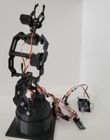
Fig.1 Revyn Arm Hardware Design.
Forward Kinematics
Forward kinematics is the process of interpreting physical constraints for a rigid body
and how free variables between rigid bodys affect their geometric positions in 3D space.
In this case, we have 6 joints meaning we have 6 free angle variables (θ1,θ2,θ3,θ4,θ5,θ6) that determine what the
final position and orientation of the end effector will be relative to the base of the robot.
We will construct a relationship between the base and end effector using these variables.
The method I will be using utilizes Homogeneous Frame transformations
and DH parameters.
To briefly summarize what this all means: we will create a frame at all 6 joints and at the base and at the end effector.
A frame is an object that holds position information and orientation information. We identify frames by using the
fixed lengths of the robot arms up to the frame position and identifying that position by using the joint variables assigned
to the joints up to the joint of interest.
When we use DH paramters to help find these frames, we have a set of rules on how these frames are likely
to be positioned relative to each other. To describe the DH parameter process in short, we will always have the frame's Z axis pointing along the axis of rotation
for the respective joint. When we move from frame to frame along the robot, we only ever rotate or translate about Z
or X. Never Y. Building the FK this way is not always necessary, but in my opinion this makes the determination of the FK and IK easier in the future.
It's not critical to understand all of these details, but if you follow along it will help you see why we make certain decisions.
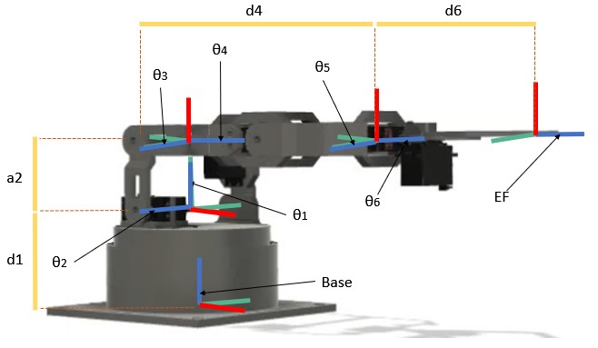
Fig.2 Revyn Arm with DH parameters.
We might define the relative 0° positions of the joints as we see in figure 2. The frames follow the pattern
with x axis-red, y axis-green, and z axis-blue. We will say that
all the joints can move +/- 90° except for joint 3 which can move between [0,180]°.
The lengths of the joints on the robot are as follows as seen in figure 2: d1 = 88.95mm a2 = 53.86mm d4 = 142.18mm d6=201.88mm
To start the FK process, we draw the frames where they should lie on the robot and collect the DH parameters to make those frames possible.
Joint n → Joint m
Z Rot (θ)
Z Trans (d)
X Trans (a)
X Rot (α)
Base (0) to Joint 1
θ1
d1
0
0
Joint 1 to Joint 2
θ2
0
0
π/2
Joint 2 to Joint 3
π/2, θ3
0
a2
0
Joint 3 to Joint 4
θ4
0
0
π/2
Joint 4 to Joint 5
θ5
d4
0
−π/2
Joint 5 to Joint 6
θ6
0
0
π/2
Joint 6 to EF
0
d6
0
0
The solution is lengthy and unintuitive to observe, but the results have been made and presented in code. The resultant symbolic forward kinematics result can be found in FK_Revyn.m and
MATLAB derivation is found in FK derivation.
Inverse Kinematics
Inverse kinematics is similar to forward kinematics in that we still want to describe the position and orientation of the end effector in 3D space relative to the base of the robot.
However with inverse kinematics, we have the goal end effector's position and orientation, but not the specific joint angles of the robot required to achieve them.
Identifying the correct joint angles is a difficult problem, and often times there is either no solution or an infinite amount of solutions.
In my approach to inverse kinematics we will address finding the most simple solution using a geometric approach. I say simple to imply that with the geometric approach you
may still find one or multiple soltuions, but if multiple solutions are returned, we will take whatever the first returned data point would be by our functions solve for the solution (e.g. If acos(0) = 0 or 180, we will take 0).
Then we will check if the solution we found is right, and if it is wrong we will take the second, or third, and so on.
We will assume that there are 6 unknowns (the six joint variables), and 6 knowns (position x,y, and z, and orientation in Euler ZYZ rotation form)
The geometric approach, as opposed to a numerical approach, is developed by investigating the geometric relationships between joint angles and robot arm lengths. We can often
obtain joint values soley by projecting triangles at different perspectives of the robot arm while the end effector and base are held at particular orientations and positions.
The actual derivation of the inverse kinematics is quite lengthy, and many researchers have identified
the solution to this problem in their works with similarly shaped robots [123]. My solution uses the same ideas and formulas.
For the derivation of my inverse kinematics see Ik derivation.
For the complete IK function see IK_Revyn.m
The IK_Revyn function accepts a Homogenous frame transform describing the end effector relative to the base.
Then it breaks the frame into a position vector and 3 ZYZ euler angles. We start the inverse operation with joint 1.
Joint 1 is found by using the law of cosines between the position of the base and the point of joint 5. The point of
joint 5 is found first by assuming the orignal orientation of the given Homogenous frame has the same orientation of the
frame at frame 6. With this assumption the position at frame 6 is just the norm of d6 vector subtracted in the orientation of the given end effector frame.
With joint 1 obtained we can find joints 2 and 3 using the law of cosines in a similar manner to the position of frame 6 at joint 5.
There are many conditions to observe in order to ensure our calculations with acos or atan2 return the angle in the correct
quadrant. See the code for these conditions.
Before we find joint 4, we will look for joint 5. We will find joint 5 again with the law of cosines, but instead we will
use the triangle formed by the point at joint 3 and the point at the end effector. Then joint 4 can be found by looking down the z axis of frame 4
taking the atan2 of the end effector x and y positions relative to the position and orientation of joint 4. Joint 6 is then found to be
the angle that is the resulting difference between the 0 angle at joint 6 and the angle required to be in the orientation for the goal given frame.
A final refinement to the algorithm was to observe the configuration of the robot after finding a possible set of joint angles.
It was deemed that if the position of joint 3 relative to the base was lower in the z axis than joints 2 and 5 then the configuration was
plausibly elbow down. This creates an unfavorable condition where the robot is likely to hit an obstable during movement, pass through areas
where the joint angles are tight, or apply high torque loads on the servos(which are already struggling to bear the full weight of the arm). When it
was observed that the arm was elbow down by investigating the relative position of joint 2, 3, and 5 the algorithm would then attempt
to change the joint angles for 2, 3, 5, 4, and 6 to achieve the same position and orentation of the end effector with the elbow up. See the code for the
methodology.
With the IK algorithm efficiently applied, I performed unit testing on my IK and FK functions to make sure they worked for all cases.
I developed some constraints based on real world physics. Unit tests would be performed on randomly generated sets of joint angles. These joint
angles would be within the acceptable range of joint angles for each joint. Then those joint angles would be fed to the FK_Revyn function
and the position of the resulting frame would be tested to ensure it's within range of the robot. Then with the output frame of FK_Revyn, we feed the frame back
to the IK_Revyn function. If the output joint angles return the same set of joint angles we started with or (if elbow up compenstated) another regenerated frame using FK_Revyn has the orientation and position
as the other genearated frame, then the case was a success. In testing, 100,000 different random sets of joint values were tested within the possible range.
All 100,000 were successful at returning possible joint angles to achieve the frame.
100,000 unit tests — all passed. Random joint angle sets were generated within the robot's physical limits, fed through FK to produce goal frames, then fed back through IK. Every case returned a valid configuration matching the original frame.
The positions of the tested frames generated the spherical shape seen in figure 3.
Fig.3 Unit testing random point generation, axis in mm.
We see a hollow portion in the sphere on the right of figure 3 because the robot cannot pass through itself, and the restricted +/- 90° joint limit on most joints doesn't allow
the robot to extend much towards its own base. The robot also cannot move past the zero Z plane as then it would be hitting the table. All cases outside of these areas were successful.
A final unit test for a handful of end cases (all joints zero, home position, singularities, etc.) were tested as well to make sure the robot returned a plausable set of joint angles.
See the script IK_Unit_Testing.m
Jacobian
To assess the potential for the robot approaching a singularity, and to see how manipulable the robot is in a given configuration we need
the jacobian.
The jacobian can found very easily with the symbolic form of the forward kinematics. We find J, the jacobian by
understanding the relationship between the jacobian and the end effector relative to the base. We refer to this particular jacobian as the spatial jacobian.
From the perspective of the base what would be the instantaneous percieved velocity should the robot move in any direction for each joint.
We find the jacobian then, by taking the derivative of the forward kinematics with respect to each joint angle. Then to see
the change relative to the base, we multiply the resultant derivative by the inverted matrix of the general forward kinematics.
The math may have been hard to follow, but check my JacobianDerivation.m and Jac_Revyn.m script where the
symbolic solution is kept for more details.
If we take the determinate of the jacobian we can assess the robots potential for reaching a local singularity. If the
determinant is close to 0 we are close to a singularity and should stop or quickly change course or the robot could reach
uncontrollable speed, commands, or behavior.
With FK, IK, and the Jacobian tools in place we could confidently move the robot to arbitrary points and orientations within the reachable workspace.
Using the script Revyn_Controller_FK_Proving the robot will be
moved to several locations within the workspace that were calculated using FK and then achieved through IK. The jacobian will ensure the robot moves through no singularity and
is applied in the FK and IK scripts. Using the same arduino control script from the first part of the project, RevynMat2ArdController.ino,
now in conjunction with MATLAB serial communication, I could assign the 6 joint angles calculated by the IK to the robot. See the next video for the script in action. The goal frame will be displayed on the left, and the robot will attempt to reach it on the right.
Linear Trajectory Planner
A really cool proof of concept idea is a linear trajectory planner.
With the robot able to follow commands, a useful tool is for it to follow a set of path commands that would
be more useful for automation. At least a little more useful than "Go to arbitrary A, okay now go to arbitrary B". We can control the orientation at the end effector, and a planner can be a little smarter and more efficient this way.
A linear trajectory planner observes the robot's position between two joints and attempts to move all of the joints so that the robot can move from point A to point B, but while maintaining the same orientation.
My robot struggles to keep power and torque engaged for really precise movements, but the mathematics and code show in simulation this can very easily be achieved.
I decided to use a step size divider that takes the path Euclidian distance between the two points (current and desired) and divdes the distance up into 2mm intervals. The robot then
moves n number of steps in 2mm intervals towards that point while maintaining the original end effector orientation.
You can see the details of how this planner works in my Lin_Traj_Revyn.m function.
I thought it would be awesome to have he robot move 4 times with a pen attached to the end effector. I would have it draw a line, and then in another test I would have it draw a rectangle.
You can see the end effector in the videos here doing fairly well to achieve the rectangular trajectories, but because of the joint angle limits and torque troubles it clearly struggles in some cases to actually draw a straight line and keep the pen tightly held.
The first video shows the robot drawing a line, then moving up and over back down to the starting spot.
The second video shows the robot drawing a rectangle. The simulation for the planned trajectories is shown first and then executed on the hardware.
Clearly there are many details to work out in the next iteration of this robot design,
however I feel that I was able to prove to myself that it is feasible to create an affordable 6 DOF robot with some degreee of accuracy and usefullness.
I think I could invest in some better motors and spend some more time tweaking the design of the hardware and control code, but currently the robot is functional and it has proved what I wanted it to.
In future work I am curious to see if I could apply other control or computer vision projects to my robot. I would love to slap a camera on the end and do hand eye calibration or something like that.
Stay tuned.
Resources
All source code for this project can be found on my github page.